In a recent post, we considered the history of the infinitesimal in calculus, from its central and controversial role in the original formulations of Newton and Leibniz to its banishment in the 19th century through the introduction of the limit. Today, we move forward to the mid-20th century, when the use of infinitesimals in calculus was finally put on a rigorous (and elegant) foundation by Abraham Robinson and his development of what came to be known as non-standard analysis.
Abraham Robinson
The basic idea is as follows: first, we will construct an extension of the standard real numbers, which will be called the “hyperreals.” The hyperreals will contain all of the standard real numbers but will also contain infinitesimal and infinite elements. Then, to perform basic calculus computations (such as taking derivatives), we will make use of the infinitesimals in the hyperreals and then translate the result back to the familiar world of the standard real numbers.
Let us now construct the hyperreals, which we denote by . To do this, let be any non-principal ultrafilter on . Let be the set of all functions from to . If and are elements of , then we say if and take the same values on a large set, or, to be more precise, if .
Speaking somewhat imprecisely, the hyperreals are the members of , where we say that two elements are in fact the same hyperreal if . (Speaking more precisely for those familiar with the terminology, the hyperreals are the equivalence classes of modulo the equivalence relation .) We want to think of the hyperreals as extending the standard reals, , so, if , then we identify with the constant function , defined so that for all .
We also want to be able to do everything with that we can do with . For example, we want to be able to say if one hyperreal is less than another, and we want to be able to add, subtract, multiply, and divide hyperreals. We do this as follows.
First, for , we say if . We similarly define , , and . Since is an ultrafilter, if , then exactly one of the following three statements is true:
Thus, we can order the hyperreals by (we haven’t shown that is in fact a linear ordering on the hyperreals; one piece of this will be done below and the rest left to you). Moreover, this ordering extends the usual ordering of the real numbers, since, if and , then clearly .
The arithmetic operations are defined pointwise. For example, is defined to be the function from to such that, for all , . Subtraction, multiplication, and division are defined in the same way. With division, we must be slightly careful with regards to division by zero. The details are unimportant for us, but let me just say that we can define the quotient for any provided that . In order to check that these operations are in fact well-defined, we would need to show, for instance, that, if and , then , and so on. I will leave this to the interested reader.
Here’s another imprecisely stated and important fact about the relationship between and : a first-order sentence is true about if and only if it is true about . I will not define ‘first-order sentence’ here, but let me illustrate this by an example. We know that , the usual ordering of the real numbers, is transitive, i.e. if and , then (in fact, transitivity is one of the requirements for being called an ‘ordering’). Let us show that is also transitive.
To do this, consider such that and . We must show that . Let and . Since and , we know that both and are in . Since is an ultrafilter, this means that . If , then and , so, by the transitivity of , we have . Let . We have shown that and . Therefore, , so .
Here’s a slightly more complex example: ‘for every , if , then there is such that .’ This is of course true in . To show that it is true in , suppose we are given such that . We must find such that . Note that, since , there is a set such that, for every , . Thus, by the existence of square roots in for every , there is a real number such that . Define a function by letting for and for . Then, for all , , so , and we have proven that our sentence is true in .
In addition to containing all of , also contains many non-standard elements, and among these are two very interesting types of hyperreals. First, contains infinite elements, i.e. elements that are larger in magnitude than every standard real number. As an example, consider the function defined by for all . To see that is larger than every standard real number, consider a number , and let be the least natural number such that . Then, for every natural number , . Since is a non-principal ultrafilter, , so . Such an is a positive infinite element. Analogously, also contains negative infinite elements.
Second, contains infinitesimal elements, elements that are non-zero but are smaller in magnitude than any standard real number. An easy way to see this is simply to take the reciprocal of an infinite element: if is positive and infinite, then (or , more precisely) is positive and smaller than any positive real number. If is the infinite element defined above, then is the function defined by for all .
An important fact about is that, although it contains many non-standard elements, every hyperreal is either infinite or infinitely close to a standard real number (where we say that a hyperreal is infinitely close to a hyperreal if is either or infinitesimal). We can therefore define the standard part of a hyperreal (denoted by ) as follows:
if is positive and infinite, then ;
if is negative and infinite, then ;
if is finite, then is the unique such that is or infinitesimal.
We are now ready to do calculus with infinitesimals! Let us show, for example, how to compute a derivative. Recall that, in its original formulation, the derivative of a function at a real number (denoted ) was defined to be:
,
where is infinitesimal. Now that we have a solid theory of infinitesimals, this is (almost) exactly the formula we will use! The only issue is that the result of this calculation will be a hyperreal, whereas we typically want answers in the standard real numbers. Therefore, we say that , if it exists, is equal to:
,
where is an infinitesimal hyperreal. To illustrate this, let’s compute the derivative of . Let be an infinitesimal hyperreal (for example, the function given by . Then:
.
Since is infinitesimal, we have , so, as expected, .
The astute reader will note that the calculation we have done does not differ substantially from the calculation we would have carried out using the limit definition of the derivative. Although non-standard analysis has led to some new technical work, its appeal is in large part historical (setting the original formulations of Newton, Leibniz, and others on a rigorous foundation) and conceptual. Infinitesimals are (to me, at least) just nicer than limits. They seem more intuitively clear; they are more easily graspable by students; they’re more fun. And they’re made possible by the heroes of our story: ultrafilters.
I’m at a conference this week and thus will not be writing any new posts. Here are some things to think about, from Pradeep Mutalik and Quanta Magazine, until we return next week with Part B in our series on non-standard analysis.
Today, we begin a historical journey from actual infinity to potential infinity and back again. We will part ways with ultrafilters for this first leg; they will get a needed rest before making a spectacular reappearance on the return trip.
In a previous post, we discussed the use of infinitesimals by Galileo and some of his contemporaries and the controversy that they caused in the scientific and religious circles of Europe during the 17th century. At the end of the 17th century, the infinitesimal took an even larger role in mathematics as one of the central players in the calculus of Newton and Leibniz. To illustrate how infinitesimals were used, let us consider the derivative, one of the fundamental concepts of calculus.
Suppose is a function. The derivative of (which exists, provided is a sufficiently well-behaved function) measures the rate of change of the value of with respect to changes in its input. For example, suppose the variable denotes time and denotes the position of a car along a road at time . Then the derivative of at a time (denoted, in Leibniz’s notation, by ), measures the velocity of the car at time .
If is a linear function (so its graph is a straight line), then the derivative of is simply the slope of that line. In our example, this would correspond to a situation in which the car was traveling at a constant velocity. But what if is a more complicated function? In this case, a fruitful approach is to try to approximate the graph of by straight lines. (This is a common tactic in mathematics: given a complicated structure that you don’t know how to deal with, try to approximate it with simpler things that you do know how to deal with.)
In practice, this might look as follows. To find the derivative of at time , choose a time close to (but different from) , find the line connecting the points and , and find the slope of this line. Doing the algebra, this slope turns out to be:
If we rewrite as , then this becomes:
The situation is illustrated in the following picture.
The derivative of f at x is approximated by the slope of the line connecting (x, f(x)) and (x+h, f(x+h)).
The smaller becomes, the closer the slope of the line between and gets to the actual derivative of at (which is the slope of the line tangent to the curve at the point . Therefore, one might think, in order to find the true derivative of , we just have to take to be really small. How small is this? Well, it certainly needs to be smaller in magnitude than every positive real number since, as the picture above illustrates, taking to be a non-zero real number just gives an approximation (though an arbitrarily good one) to the actual derivative. However, it cannot be equal to , since, if , then
which is of course undefined. The obvious answer, to those who accept the use of such things, at least, is to let be a non-zero infinitesimal. This is essentially the approach taken by Newton and Leibniz. (I am of course simplifying things, but this is the general idea).
The formulation of calculus by Newton and Leibniz was a great success and led to many further advances in science and mathematics, but the controversy surrounding the use of infinitesimals did not go away. As we mentioned in the earlier post, indiscriminate use of infinitesimals often led to paradox. There were also attacks on ontological grounds. Opponents of the use of infinitesimals claimed that their proponents wanted things both ways: on the one hand, infinitesimals should have positive magnitude to avoid undefined expressions such as ; on the other hand, this positive magnitude should be smaller than any real positive magnitude. These two demands seemed contradictory. In addition, there is the observation that, if is a positive infinitesimal, then would be a positive infinite number, clashing with the orthodoxy of the time that actual infinity should not be present in mathematics.
These objections essentially amounted to an appeal to what came to be known as the Archimedean property as applied to the set of real numbers. Briefly, the Archimedean property states that there are no infinite or infinitesimal elements in a given structure. More precisely (and in the context of the real numbers (it is the same for any ordered field, for example)), the Archimedean property states that, if and are any two positive numbers, then there is a natural number such that . The Archimedean property appeared in Euclid’s Elements and was given its name by mathematician Otto Stolz in the 1880s. Stolz did much work on extensions of the real numbers which do not satisfy the Archimedean property. Interestingly and rather surprisingly, Cantor called this work an “abomination” and published an attempted sketch of a proof of the non-existence of infinitesimals.
An illustration of the Archimedean property, which essentially states that any positive magnitude can be covered by finitely many copies of any other. Here, 4 copies of A are sufficient to cover B.
The standard real numbers, , satisfy the Archimedean property. However, if is extended to include infinitesimals, then the Archimedean property fails. To see this, let be a positive infinitesimal, and let . Since is an infinitesimal, we must have for every natural number , so for all natural and thus and witness the failure of the Archimedean property.
One of the most prominent opponents of infinitesimals was Bishop Berkeley, who, in 1734, published The Analyst, an attack on the foundations of infinitesimal calculus with the wonderful subtitle, A DISCOURSE Addressed to an Infidel MATHEMATICIAN. WHEREIN It is examined whether the Object, Principles, and Inferences of the modern Analysis are more distinctly conceived, or more evidently deduced, than Religious Mysteries and Points of Faith. In the following memorable passage, Berkeley calls into question the nature and existence of infinitesimals (in what follows, ‘fluxions’ refers to a definition of Newton closely related to the derivative):
And what are these Fluxions? The Velocities of evanescent Increments? And what are these same evanescent Increments? They are neither finite Quantities nor Quantities infinitely small, nor yet nothing. May we not call them the ghosts of departed quantities?
Bishop Berkeley
Newton, Leibniz, and like-minded mathematicians of course defended their use of infinitesimals. Leibniz explicitly justified their use in his Law of Continuity, expressed in a manuscript in 1701:
In any supposed continuous transition, ending in any terminus, it is permissible to institute a general reasoning, in which the final terminus may also be included.
And more plainly in a letter from 1702:
The rules of the finite are found to succeed in the infinite.
The debate over infinitesimals was undoubtedly a good thing for mathematics, as it inspired mathematicians to work to put calculus on rigorous foundations. This was largely done in the 19th century, as the actual infinities of infinitesimals were replaced by the potential infinities of limits, and the definition of the derivative settled into the form familiar to students of calculus ever since:
In calculating such a limit, one considers the behavior of as becomes arbitrarily close, but not equal, to . Importantly, these values of are all standard real numbers and not infinitesimal. Infinitesimals themselves came to be seen as something like a useful but foundationally suspect fiction, a heuristic that helped lead to the great achievements of calculus but which had properly been discarded upon the rigorous founding of calculus in the language of limits.
This would be a natural ending point for our story. Indeed, this is how the story went for about 100 years, and calculus as taught in most schools today is hardly changed from its 19th century formulation. However, surprises awaited in the mid-20th century, when the use of infinitesimals in calculus was finally put on a rigorous foundation and Newton, Leibniz, and other proponents were, in a sense, vindicated. We’ll have that story in our next installment.
Today, we take a look at infinite objects that have actually found a use in our finite world. (Or, more accurately but less spectacularly, their finite approximations have found a use.)
Take a look at these two videos from 3Blue1Brown, the first giving some background on and a hypothetical application of space-filling curves, and the second indulging in some space-filling play. Enjoy!
Ramsey theory is an area of the mathematical field of combinatorics. Its slogan could be, “In a large enough structure, order must arise.” It is named after Frank Ramsey, student of Keynes, friend of Wittgenstein, brother of the future Archbishop of Canterbury, who did seminal work in the area before tragically dying at the age of 26.
Frank Ramsey
You may have heard this one. Suppose you’re throwing a party. You don’t really know whether the people you’re thinking of inviting know one another, and you want to make sure that, at the party, there are either three people who mutually know one another or three people who mutually do not know one another (as everyone knows, a party is doomed to be a failure if this doesn’t happen). What is the least number of people you need to invite to make sure this happens?
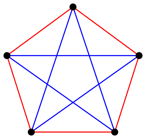
The answer is 6. We need to prove two things. First, 5 is not enough. To see this, consider the following picture. Suppose each of the dots is a person at your party, and two people are connected with a red edge if they know one another and a blue edge if they do not know one another. If you get unlucky enough to invite exactly such a configuration of five guests, you will not have a group of three that mutually know one another nor a group of three that mutually do not know one another.
A disastrous party.
We next need to show that 6 is indeed sufficient. I’ll leave this as an exercise for the reader. It’s fun! You should do it.
(What is the least number of people you need to invite to ensure a group of four people who mutually know one another or a group of four people who mutually do not know one another? 18. What about for groups of five? Nobody knows (or, if they do, they haven’t told me), but it’s between 43 and 49.)
This is the standard introductory theorem in Ramsey theory. To state more general results, it will be helpful to have some notation.
Notation: Suppose is a set and is a natural number. Then denotes the set of all -element subsets of , i.e. .
Definition: Suppose are sets, is a natural number, and . If , then we say is homogeneous for if there is a single element such that, for all , .
The existence of a large homogeneous set for a given function is an example of a certain amount of order existing in . Therefore, a typical theorem in Ramsey theory may be something like this: If is sufficiently large with respect to , is a certain natural number, and is any function from to , then there is a large homogeneous set for . Of course, ‘sufficiently large’ and ‘large’ would need to be made precise in the statement of an actual theorem.
With this language, we can restate our party theorem as follows: Suppose , , and . Then has a homogeneous set of size . Moreover, this is no longer true if we just assume .
Finite Ramsey theory is a fascinating and rich subject, and I encourage readers to learn more about it. Given the domain of this blog though, we want to consider Ramsey theory on infinite sets. The seminal result in this direction is, naturally, the Infinite Ramsey Theorem, proven by Ramsey in 1930.
Infinite Ramsey Theorem: Suppose and . Then there is an infinite homogeneous set for .
Proof: If either or is equal to , then the theorem is trivial. We prove the theorem for the case and an arbitrary value of . The general statement is proven in a similar way (with some additional care taken at certain points) by induction on .
Let be a non-principal ultrafilter on . We will consider elements of as ordered pairs such that . For each and , let be the set of such that and . Since is a non-principal ultrafilter and , we may fix a natural number such that . Again using the fact that is a non-principal ultrafilter, we may find a set and a fixed natural number such that, for all , .
We now construct an infinite set such that, for every with both and in , we have . We will do this one element at a time, enumerating in increasing order as . To start, let be the least element of . Next, find such that . Since and are in , such an exists and, as , we have . Next, find such that . As before, such an always exists and . Keep going in this fashion. Namely, if and we have already defined , then find such that . Since this is an intersection of finitely many sets, all of which are in , we can always find such an and, for all , we have . Thus, we can continue for infinitely many steps, completing the definition of and therefore the proof of the theorem.
Remarks: The use of an ultrafilter here is not really necessary but makes the proof a little slicker. It also raises an interesting question related to the notion that Ramsey theory is about finding large homogeneous sets. Recall that ultrafilters can be thought of as specifying which subsets of a given set should be considered to be ‘large.’ In the Infinite Ramsey Theorem, we were able to obtain an infinite homogeneous set, but can we always find a homogeneous set ? This question motivates the following definition.
Definition: Let be a non-principal ultrafilter on . is called a Ramsey ultrafilter if, for all natural numbers and every function , there is a set that is homogeneous for .
So our question becomes: are all non-principal ultrafilters on Ramsey ultrafilters? The answer to this is: “No.” There are always non-principal ultrafilters on that are not Ramsey ultrafilters.
So the next question, of course, is: are there any Ramsey ultrafilters? This turns out to be the interesting question, and the answer is: “It depends.” The existence of Ramsey ultrafilters is independent of the usual axioms of set theory (the axioms of ZFC). Namely, it is consistent with the axioms of ZFC that Ramsey ultrafilters exist, but it is also consistent with ZFC that Ramsey ultrafilters do not exist.
Infinite Ramsey theory has been in the news lately due to a recent breakthrough in reverse mathematics by Ludovic Patey and Keita Yokoyama. Let me try to briefly (and therefore rather imprecisely) explain their result, with the caveat that I am in no way an expert in reverse mathematics.
As I mentioned, the standard proofs of the Infinite Ramsey Theorem are pretty similar for the cases and . This should make a certain amount of sense, since the statements for and are quite similar. However, in another sense, this is somewhat misleading, as the standard proof of the Infinite Ramsey Theorem takes place in the setting of the axioms of set theory (ZFC), and these axioms may be much more powerful than necessary. Reverse mathematics attempts to classify theorems by exactly how much one needs to assume (beyond some fixed, very weak base system (known as )) to prove them. A hierarchy of systems extending has been uncovered through the attempt to pin down the logical strengths of various theorems. An interesting dividing line in the set of these systems is between those that are ‘finitistic’ (essentially, those that do not rely on the existence of infinite sets) and those that are ‘infinitistic.’ The strongest finitistic system in widespread use is ‘primitive recursive arithmetic,’ or ‘PRA.’ A theorem is thus called ‘finitistically reducible’ if it is finitistically reducible to PRA (roughly, if it can be proven without the use of infinite sets).
It was known already that the instance of the Infinite Ramsey Theorem with and is not finitistically reducible. This makes a certain naive, intuitive sense, as the conclusion of the theorem asserts the existence of an infinite homogeneous set. Patey and Yokoyama’s surprising result is that the instance of the Infinite Ramsey Theorem with and is finitistically reducible. Unlike the infinite homogeneous set generated by the case, that generated by the case is, in a sense, simple enough that any consequence of its existence can be obtained purely finitistically.
For those of you who want to read more about this interesting result, there’s a decent article about it in Quanta Magazine, and Patey and Yokoyama’s paper can be found here.


;
;
is


 is a function. The derivative of
  denotes the position of a car along a road at time
  (denoted, in Leibniz’s notation, by
  ), measures the velocity of the car at time
  close to (but different from)
  and
and  , and find the slope of this line. Doing the algebra, this slope turns out to be:
 , then this becomes:
 and
and  gets to the actual derivative of
  , then
 ; on the other hand, this positive magnitude should be smaller than any real positive magnitude. These two demands seemed contradictory. In addition, there is the observation that, if
  would be a positive infinite number, clashing with the orthodoxy of the time that actual infinity should not be present in mathematics.
 such that
  . The Archimedean property appeared in Euclid’s Elements and was given its name by mathematician Otto Stolz in the 1880s. Stolz did much work on extensions of the real numbers which do not satisfy the Archimedean property. Interestingly and rather surprisingly, Cantor called this work an “abomination” and published an attempted sketch of a proof of the non-existence of infinitesimals.
 . Since
  for every natural number
  for all natural
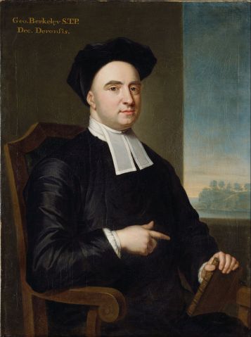

 as
as 
![[X]^n](https://s0.wp.com/latex.php?latex=%5BX%5D%5En&bg=fffdfd&fg=606666&s=0&c=20201002) denotes the set of all
denotes the set of all ![[X]^n = \{Y \subseteq X \mid |Y| = n\}](https://s0.wp.com/latex.php?latex=%5BX%5D%5En+%3D+%5C%7BY+%5Csubseteq+X+%5Cmid+%7CY%7C+%3D+n%5C%7D&bg=fffdfd&fg=606666&s=0&c=20201002) .
. are sets,
 ![f:[X]^n \rightarrow Y](https://s0.wp.com/latex.php?latex=f%3A%5BX%5D%5En+%5Crightarrow+Y&bg=fffdfd&fg=606666&s=0&c=20201002) . If
. If  , then we say
  is homogeneous for
  such that, for all
 ![A \in [H]^n](https://s0.wp.com/latex.php?latex=A+%5Cin+%5BH%5D%5En&bg=fffdfd&fg=606666&s=0&c=20201002) ,
,  .
. ,
,  ,
,  , and
, and ![f:[X]^2 \rightarrow Y](https://s0.wp.com/latex.php?latex=f%3A%5BX%5D%5E2+%5Crightarrow+Y&bg=fffdfd&fg=606666&s=0&c=20201002) . Then
. Then  . Moreover, this is no longer true if we just assume
  .
. and
and ![f:[\mathbb{N}]^n \rightarrow \{1, \ldots, k\}](https://s0.wp.com/latex.php?latex=f%3A%5B%5Cmathbb%7BN%7D%5D%5En+%5Crightarrow+%5C%7B1%2C+%5Cldots%2C+k%5C%7D&bg=fffdfd&fg=606666&s=0&c=20201002) . Then there is an infinite homogeneous set
. Then there is an infinite homogeneous set  for
for  is equal to
  , then the theorem is trivial. We prove the theorem for the case
  and an arbitrary value of
 ![[\mathbb{N}]^2](https://s0.wp.com/latex.php?latex=%5B%5Cmathbb%7BN%7D%5D%5E2&bg=fffdfd&fg=606666&s=0&c=20201002) as ordered pairs
as ordered pairs  such that
  . For each
  and
and  , let
, let  be the set of
  such that
  . Since
  , we may fix a natural number
  such that
  . Again using the fact that
  and a fixed natural number
  such that, for all
  ,
,  .
. such that, for every
  and
and  in
in  . We will do this one element at a time, enumerating
  . To start, let
  be the least element of
  . Next, find
  such that
  . Since
  are in
  exists and, as
  , we have
  . Next, find
  such that
  . As before, such an
  always exists and
  . Keep going in this fashion. Namely, if
  and we have already defined
  , then find
  such that
  . Since this is an intersection of finitely many sets, all of which are in
  and, for all
  , we have
  . Thus, we can continue for infinitely many steps, completing the definition of
  ? This question motivates the following definition.
 and every function
  and
and  . This should make a certain amount of sense, since the statements for
  )) to prove them. A hierarchy of systems extending
  is not finitistically reducible. This makes a certain naive, intuitive sense, as the conclusion of the theorem asserts the existence of an infinite homogeneous set. Patey and Yokoyama’s surprising result is that the instance of the Infinite Ramsey Theorem with