Hello! It’s been over a year since my last post; I took some time off as I moved to a new city and a new job and became generally more busy. I missed writing this blog, though, and recently I found myself reading about supertasks, tasks or processes with infinitely many steps but which are completed in a finite amount of time. This made the finitely many things I was doing seem lazy by comparison, so I think I’m going to try updating this site regularly again.
The first supertasks were possibly those considered by Zeno in his paradoxes of motion (which we’ve thought about here before). In the simplest, Achilles is running a 1 kilometer race down a road. To complete this race, though, Achilles must first run the first 1/2 kilometer. He must then run the next 1/4 kilometer, and then the next 1/8 kilometer, and so on. He must seemingly complete an infinite number of tasks just in order to finish the race.
If this idea leaves you a bit confused, you’re not alone! It seems that the same idea can be applied to any continuous process; first half of the process must take place, then the next quarter, then the next eighth, and so on. How does anything ever get done? Is every task a supertask?
Supertasks reemerged as a topic of philosophical study in the mid-twentieth century, when J.F. Thomson introduced both the term supertask and a new example of a supertask, now known as Thomson’s Lamp: Imagine you have a lamp with an on/off switch. Now imagine that you switch the lamp on at time t = 0 seconds. After 1/2 second, you switch the lamp off again. After a further 1/4 second, you switch the lamp on again. After a further 1/8 second, you switch the lamp off again, and so on. After 1 full second, you have switched the lamp on and off infinitely many times. Now ask yourself: at time t = 1, is the lamp on or off? Is this even a coherent question to ask?
We’ll have more to say about this and other supertasks in future posts, but today I want to present a particularly elegant supertask introduced by Jon Perez Laraudogoitia in the aptly named paper “A Beautiful Supertask”, published in the journal Mind in 1996. Before describing the supertask, let me note that it will obviously not be compatible with our physical universe, or perhaps any coherent physical universe, for a number of reasons: it assumes perfectly elastic collisions with no energy lost (no sound or heat created, for instance), it assumes that particles with a fixed mass can be made arbitrarily small, it assumes that nothing will go horribly wrong if we enclose infinitely much matter in a bounded region, and it neglects the effects of gravity. Let’s put aside these objections for today, though, and simply enjoy the thought experiment.
Imagine that we have infinitely objects, all of the same mass. Call these objects m1, m2, m3, and so on. They are all arranged on a straight line, which we’ll think of as being horizontal. To start, each of these objects is standing still. Object m1 is located 1 meter to the right of a point we will call the origin, object m2 is 1/2 meter to the right of the origin, object m3 is 1/4 meter to the right of the origin, and so on. (Again, we’re ignoring gravity here. Also, so that we may fit these infinitely many objects in a finite amount of space, you can either assume that they are point masses without dimension or you can imagine them as spheres that get progressively smaller (but retain the same mass) as their index increases.) Meanwhile, another object of the same mass, m0, appears to the right of m1, moving to the left at 1 meter per second. At time t = 0 seconds, it collides with m1.
Our system immediately before t = 0.
What happens after time t = 0? Well, since we’re assuming our collisions are perfectly elastic, m0 transfers all of its momentum to m1, so that m0 is motionless 1 meter from the origin and m1 is moving to the left at 1 meter per second. After a further half second, at t = 1/2, m1 collides with m2, so that m1 comes to rest 1/2 meter from the origin while m2 begins moving to the left at 1 meter per second. This continues. At time t = 3/4, m2 collides with m3. At time t = 7/8, m3 collides with m4, and so on.
Where are we after 1 full second? By time t = 1, each object has been hit by the previous object and has in turn collided with the next object. m0 is motionless where m1 started, m1 is motionless where m2 started, m2 is motionless where m3 started, and so on. Our entire system is at rest. Moreover, compare the system {m0, m1, m2, …} at t=1 to the system {m1, m2, m3, …} at t=0. They’re indistinguishable! Our initial system {m1, m2, m3, …} has absorbed the new particle m0 and all of its kinetic energy and emerged entirely unchanged!
Things become seemingly stranger if we reverse time and consider this process backwards. We begin with the system {m0, m1, m2, …}, entirely at rest. But then, at t = -1, for no apparent reason, a chain reaction of collisions begins around the origin (“begins” might not be quite the right terms — there’s no first collision setting it all off). The collisions propagate rightward, and at t = 0 the system spits out particle m0, moving to the right at 1 meter per second, while the system {m1, m2, m3, …} is now identical to the system {m0, m1, m2, …} at time t = -1. The ejection of this particle from a previously static system is an inexplicable event. It has no root cause; each collision in the chain was caused by the one before it, ad infinitum. A moving object has seemingly emerged from nothing; kinetic energy has seemingly been created for free.
(Friendly note to the reader before we begin: If you’re looking for music to listen to while reading this post, just scroll to the bottom…)
The Spallation Neutron Source (SNS), at Oak Ridge National Laboratory in Tennessee, provides the world’s most intense pulsed neutron beams for scientific research. By accelerating proton pulses and directing them towards a mercury target, the laboratory ejects neutrons from the target. By measuring the energies and angles of these scattered neutrons, scientists can uncover information about the magnetic and molecular structure of various materials.
Pulses at the SNS are grouped into super-cycles, each 10 seconds long and consisting of 600 pulses. Commonly, experimenters will want to perform a particular action on a fixed number of pulses (, say) during each super-cycle and will want to have the executions of the actions spaced as evenly as possible across time. If evenly divides 600, then the solution to this problem is trivial: just perform the action on pulses . If does not evenly divide 600, though, then the solution is not as obvious.
This is of course a special case of a general problem: Given cycles of length , how can events be spaced as evenly as possible across a single cycle? (Naturally, we should have here.) As seen above, the problem is trivial if evenly divides , so we shall assume this is not the case. In fact, we shall assume that and are relatively prime, i.e., that they have no common positive divisors other than 1. We will also assume that , since it is also trivial to evenly distribute one event across a cycle.
This exact problem was tackled by E. Bjorklund, motivated by timing questions at the SNS. In this paper, he presents an algorithm for generating solutions. For ease of notation, let us denote a cycle by a sequence of 0s and 1s, with a 1 representing an event taking place and a 0 representing an event not taking place. For definiteness, we will always start the sequence with a 1, but, because we are dealing with cyclic phenomena, we will consider two “rotations” of the same base sequence to be the same. For example, we consider 10010 and 10100 to be the same, since the second is just the first “rotated” (and wrapped around) three spaces to the right.
We will not give a formal account of Bjorklund’s algorithm here, but we will illustrate it with an example that we hope will indicate how to carry it out in general. Suppose we are given the specific problem of evenly spacing eight events in a cycle of length thirteen. Our final sequence will thus have eight 1s and five 0s. We start with thirteen individual sequences, each of length one, with all of the 1s first and then all of the 0s:
You will notice that we have two different sequences in this list ([1] and [0], here). This will be true for every step of the algorithm. In the next step, we take all instances of the second sequence ([0], here) and append them in turn to instances of the first sequence. Since there are five instances of the second sequence, five instances of the first sequence will become longer, and we obtain:
[10] [10] [10] [10] [10] [1] [1] [1]
We again have two different sequences ([10] and [1]). And we again take all instances of the second sequence and append them in turn to instances of the first sequence, obtaining:
[101] [101] [101] [10] [10]
Repeating this process again yields:
[10110][10110][101]
Technically, since there is only one instance of the second sequence in this stage, we could stop here and just append all of the sequences in order to obtain the correct solution, but let us continue for illustration’s sake. Next, we get:
[10110101][10110]
And, finally:
[1011010110110}
(which is just a rotation of what we would have gotten two stages earlier: [1011010110101]). Thus, the optimal way of evenly distributing eight events in a single cycle of length 13 is given by the sequence 1011010110110. A similar process will yield the correct answer in any other specific instance of this problem.
(The astute reader might have noticed that this algorithm bears a resemblance to Euclid’s famous algorithm for calculating the greatest common divisor of two positive integers. This is not a coincidence.)
You might be slightly disturbed by my lack of rigor at this point. Indeed, there are two ways in which I am slightly cheating the reader. First, I have not really said what I mean by having events be spaced “as evenly as possible.” Intuitively, 1011010110110 is more even than 111111110000, or 1101101101100, or, if one thinks about it, 1011011011010, but how do we know it is “as even as possible,” and what do we even mean by this? Second, even if I had given a rigorous definition of “evenness,” I have not proven that Bjorklund’s algorithm does in fact deliver the optimal result (again, this should be intuitively plausible, but should perhaps not be blindly accepted). I will do neither of these things here, but will instead direct the interested reader to the excellent paper, “The distance geometry of music,” by Demaine, Gomez-Martin, Meijer, Rappaport, Taslakian, Toussaint, Winograd, and Wood, from which much of this post was derived.
Unsurprisingly, the problem of evenly distributing events or items into cycles of length does not show up only in nuclear physics. Let us briefly look at a couple of other interesting appearances.
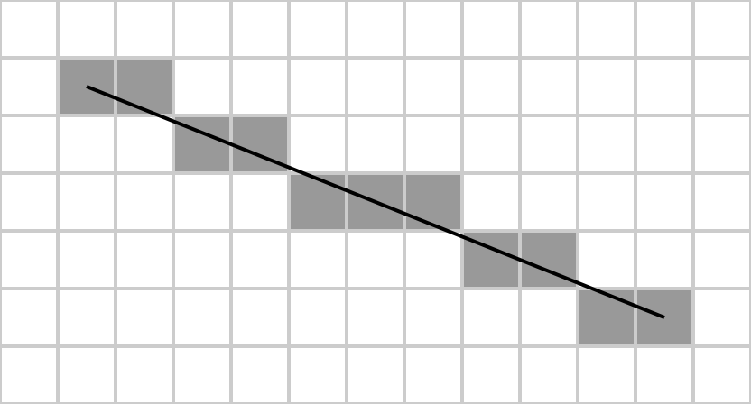
Computer graphics: Suppose you want to depict a straight line on a computer screen with a slope of . Computer screens consist of grids of pixels, so, unless the line is horizontal or vertical, it cannot be drawn perfectly straight. Here is an example of a segment of a line with slope :
A line with slope -5/11, superimposed over a pixel approximation. Created by Crotalus horridus, Public Domain
It should be clear that, at least as long as , the problem of drawing this line consists of choosing out of every horizontal spaces after which to move your line one space vertically. To make your line as straight as possible, this distribution should be as even as possible. Indeed, the situation depicted above can be represented by the sequence 10101001010, where 1 indicates a vertical shift and 0 represents the absence of a vertical shift. This is precisely the result one gets (after a rotation) if one applies Bjorklund’s algorithm to the numbers 5 and 11.
Leap year distribution: The problem of reconciling the fact that one revolution of the earth around the sun does not take an exact integer number of days with the desire to have years that last an exact integer number of days is one that affects every calendar design. It is handled particularly interestingly in the Hebrew calendar. The Hebrew calendar is a lunisolar calendar, in which each month lasts one full cycle of the moon, but in which adjustments are made so that each month occurs at roughly the same stage of the solar year during each cycle. The Hebrew calendar reconciles these two contradictory demands by having twelve months in a typical year but, during certain “leap years,” having one of these months (namely, Adar) repeated to yield a year of thirteen months. It turns out that, to keep the Hebrew calendar very close to being in sync with the solar cycles, one needs to have seven out of every nineteen years be leap years. It is also natural to want these leap years to be spaced as evenly as possible. And, indeed, the distribution of these seven leap years in nineteen-year cycles in the Hebrew calendar is given precisely by a rotation of the result of Bjorklund’s algorithm applied to the numbers seven and nineteen.
Perhaps the most interesting appearances of the problem of evenly distributing events in a cycle, though, are in music. If one thinks of a musical measure consisting of beats as being a cycle of length , of a 1 as being a note being played, and of a 0 as being the absence of a note being played, then our strings of 1s and 0s can be thought of as musical rhythms. And it turns out that applications of Bjorklund’s algorithm, when interpreted in this way, yield a startling variety of musical rhythms used in practice around the world. We end this post by presenting a few prominent examples.
In what follows, we notationally replace 1s with ‘x’s and 0s with dots. This is more conducive to following along with musical rhythms, as it is visually easier to get lost in strings of 1s and 0s than in strings of ‘x’s and dots. An ‘x’ thus denotes a note being played and a dot denotes the absence of a note being played (or, often, an ‘x’ denotes an accented beat and a dot denotes an unaccented beat). Given numbers , we denote by the result of Bjorklund’s algorithm applied to and . The sequence that follows is the rotation of this result that is actually heard in the piece of music. As before, we restrict ourselves to the interesting cases in which and are relatively prime and . (Of course, the standard waltz rhythm [x . . ], for example, would be E(1,3), and the standard backbeat rhythm [. x . x ] would be a rotation of E(2,4), but these are sort of boring in this context.)
There’s some good music here. Enjoy!
E(2,5) – (x . . x . ): “Take Five” by The Dave Brubeck Quartet.
E(3,7) – (x . x . x . . ): “Money” by Pink Floyd.
E(3,8) – (x . . x . . x . ): This is the famous tresillo rhythm, which can be heard throughout Latin American and sub-Saharan African music as well as in such songs as “Hound Dog,” “Despacito,” and the song we feature here, “Intro” by The xx.
E(5,8) – (x . x x . x x . ): This is the cinquillo rhythm, an elaboration of the tresillo that is also ubiquitous in Latin American and sub-Saharan African music. It also features prominently in “Come Out and Play” by The Offspring.
E(4,9) – (x . x . x . x . . ): This is our second track from the classic Time Out album, which was inspired by musical styles (especially time signatures) observed during travels in Europe and Asia. Brubeck saw this particular beat being played by Turkish street musicians and then used it for “Blue Rondo à la Turk” by The Dave Brubeck Quartet.
E(4,11) – (x . . x . . x . . x . ): “Outside Now” by Frank Zappa.
E(5,11) – (x . x . x . x . x . .): “Promenade” from Pictures at an Exhibition by Modest Mussorgsky.
E(7,12) – (x . x . x x . x . x . x): This is one of the most important rhythms in sub-Saharan Africa, often used as a bell pattern. It is also a common beat in the Palo music of the Caribbean. It can be heard played by the claves player in this performance by Los Calderones, which I have been listening to non-stop for the last hour. (Note also that, if one re-interprets this sequence in a harmonic rather than rhythmic setting, in which each step of the cycle represents a half-step in pitch, an ‘x’ represents the inclusion of that note in a scale, and a dot represents the exclusion of that note from a scale, then this sequence (this exact rotation, in fact) precisely corresponds to the major diatonic scale, the most common musical scale in Western music!)
E(4,13) – (x . . x . . x . . x . . . ): This rhythm can be heard in the instrumental sections of “Golden Brown” by The Stranglers.
E(5,16) – (x . . x . . x . . . x . . x . . ): This rhythm forms the basis for much bossa nova music and, when significantly slowed down, “Pyramid Song” by Radiohead.
Cover image: Detail from “Wall Drawing #260” by Sol LeWitt
Last week, we began a series of posts dedicated to thinking about immortality. If we want to even pretend to think precisely about immortality, we will have to consider some fundamental questions. What does it mean to be immortal? What does it mean to live forever? Are these the same thing? And since immortality is inextricably tied up in one’s relationship with time, we must think about the nature of time itself. Is there a difference between external time and personal time? What is the shape of time? Is time linear? Circular? Finite? Infinite?
Of course, we exist not just across time but across space as well, so the same questions become relevant when asked about space. What is the shape of space? Is it finite? Infinite? It is not hard to see how this question would have a significant bearing on our thinking about immortality. In a finite universe (or, more precisely, a universe in which only finitely many different configurations of matter are possible), an immortal being would encounter the same situations over and over again, would think the same thoughts over and over again, would have the same conversations over and over again. Would such a life be desirable? (It is not clear that this repetition would be avoidable even in an infinite universe, but more on that later.)
Today, we are going to take a little historical detour to look at the shape of the universe, a trip that will take us from Ptolemy to Dante to Einstein, a trip that will uncover a remarkable confluence of poetry and physics.
One of the dominant cosmological views from ancient Greece and the Middle Ages was that of the Ptolemaic, or Aristotelian, universe. In this image of the world, Earth is the fixed, immobile center of the universe, surrounded by concentric, rotating spheres. The first seven of these spheres contain the seven “planets”: the Moon, Mercury, Venus, the Sun, Mars, Jupiter, and Saturn. Surrounding these spheres is a sphere containing the fixed stars. This is the outermost sphere visible from Earth, but there is still another sphere outside it: the Primum Mobile, or “Prime Mover,” which gives motion to all of the spheres inside it. (In some accounts the Primum Mobile is itself divided into three concentric spheres: the Crystalline Heaven, the First Moveable, and the Empyrean. In some other accounts, the Empyrean (higher heaven, which, in the Christianity of the Middle Ages, became the realm of God and the angels) exists outside of the Primum Mobile.)
An illustration of the Ptolemaic universe from The Fyrst Boke of the Introduction of Knowledge by Andrew Boorde (1542)
This account is naturally vulnerable to an obvious question, a question which, though not exactly in the context of Ptolemaic cosmology, occupied me as a child lying awake at night and was famously asked by Archytas of Tarentum, a Greek philosopher from the fifth century BC: If the universe has an edge (the edge of the outermost sphere, in the Ptolemaic account), then what lies beyond that edge? One could of course assert that the Empyrean exists as an infinite space outside of the Primum Mobile, but this would run into two objections in the intellectual climate of both ancient Greece and Europe of the Middle Ages: it would compromise the aesthetically pleasing geometric image of the universe as a finite sequence of nested spheres, and it would go against a strong antipathy towards the infinite. Archytas’ question went largely unaddressed for almost two millennia, until Dante Alighieri, in the Divine Comedy, proposed a novel and prescient solution.
Before we dig into Dante, a quick mathematical lesson on generalized spheres. For a natural number , an -sphere is an -dimensional manifold (i.e. a space which, at every point, locally looks like -dimensional real Euclidean space) that is most easily represented, embedded in -dimensional space, as the set of all points at some fixed positive distance (the “radius” of the sphere) from a given “center point.”
Perhaps some examples will clarify this definition. Let us consider, for various values of , the -sphere defined as the set of points in -dimensional Euclidean space at distance 1 from the origin (i.e. the point (0,0,…,0)).
If , this is the set of real numbers whose distance from 0 is equal to 1, which is simply two points: 1 and -1.
If , this is just the set of points in the plane at a distance of 1 from . This is the circle, centered at the origin, with radius 1.
A 1-sphere
If , this is the set of points in 3-dimensional space at a distance 1 from the point . This is the surface of a ball of radius 1, and is precisely the space typically conjured by the word “sphere.”
A 2-sphere
0-, 1-, and 2-spheres are all familiar objects; beyond this, we lose some ability to visualize -spheres due to the difficulty of considering more than three spatial dimensions, but there are useful ways to think about higher-dimensional spheres by analogy with the more tangible lower-dimensional ones. Let us try to use these ideas to get some understanding of the 3-sphere.
First, note that, for a natural number , the non-trivial “cross-sections” of an -sphere are themselves -spheres! For example, if a 1-sphere (i.e. circle) is intersected with a 1-dimensional Euclidean space (a line) in a non-trivial way, the result is a -sphere (i.e. a pair of points). If a 2-sphere is intersected with a 2-dimensional Euclidean space (a plane) in a non-trivial way, the result is a 1-sphere (this is illustrated above in our picture of a 2-sphere). The same relationship holds for higher dimensional spheres: if a 3-sphere is intersected with a 3-dimensional Euclidean space in a non-trivial way, the result is a 2-sphere.
Suppose that you are a 2-dimensional person living in a 2-sphere universe. Let’s suppose, in fact, that you are living in the 2-sphere pictured above, with the 1-sphere “latitude lines” helpfully marked out for you. Let’s suppose that you begin at the “north pole” (i.e. the point at the top, in the center of the highest circle) and start moving in a fixed direction. At fixed intervals, you will encounter the 1-sphere latitude lines. For a while, these 1-spheres will be increasing in radius. This will make intuitive sense to you. You are moving “further out” in space; each successive circle “contains” the last and thus should be larger in radius. After you pass the “equator,” though, something curious starts happening. Even though you haven’t changed direction and still seem to be moving “further out,” the radii of the circles you encounter start shrinking. Eventually, you reach the “south pole.” You continue on your trip. The circles wax and wane in a now familiar way, and, finally, you return to where you started.
A similar story could be told about a 3-dimensional being exploring a 3-sphere. In fact, I think we could imagine this somewhat easily. Suppose that we in fact live in a 3-sphere. For illustration, let us place a “pole” of this 3-sphere at the center of the Earth. Now suppose that we, in some sort of tunnel-boring spaceship, begin at the center of the Earth and start moving in a fixed direction. For a while, we will encounter 2-sphere cross-sections of increasing radius. Of course, in the real world these are not explicitly marked (although, for a while, they can be nicely represented by the spherical layers of the Earth’s core and mantle, then the Earth’s surface, then the sphere marking the edge of the Earth’s atmosphere) but suppose that, in our imaginary world, someone has helpfully marked them. For a while, these successive 2-spheres have larger and larger radii, as is natural. Eventually, of course, they will start to shrink, contracting to a point before expanding and contracting as we return to our starting point at the Earth’s core.
Dante’s Divine Comedy, completed in 1320, is one of the great works of literature. In the first volume, Inferno, Dante is guided by Virgil through Hell, which exists inside the Earth, directly below Jerusalem (from where I happen to be writing this post). In the second volume, Purgatorio, Virgil leads Dante up Mount Purgatory, which is situated antipodally to Jerusalem and formed of the earth displaced by the creation of Hell. In the third volume, Paradiso, Dante swaps out Virgil for Beatrice and ascends from the peak of Mount Purgatory towards the heavens.
Dante’s universe. Image by Michelangelo Caetani.
Dante’s conception of the universe is largely Ptolemaic, and most of Paradiso is spent traveling outward through the larger and larger spheres encircling the Earth. In Canto 28, Dante reaches the Primum Mobile and turns his attention outward to what lies beyond it. We are finally in a position to receive an answer to Archytas’ question, and the answer that Dante comes up with is surprising and elegant.
The structure of the Empyrean, which lies outside the Primum Mobile, is in large part a mirror image of the structure of the Ptolemaic universe, a revelation that is foreshadowed in the opening stanzas of the canto:
When she who makes my mind imparadised
Had told me of the truth that goes against
The present life of miserable mortals —
As someone who can notice in a mirror
A candle’s flame when it is lit behind him
Before he has a sight or thought of it,
And turns around to see if what the mirror
Tells him is true, and sees that it agrees
With it as notes are sung to music’s measure —
Even so I acted, as I well remember,
While gazing into the bright eyes of beauty
With which Love wove the cord to capture me.
When Dante looks into the Empyrean, he sees a sequence of concentric spheres, centered around an impossibly bright and dense point of light, expanding to meet him at the edge of the Primum Mobile:
I saw a Point that radiated light
So sharply that the eyelids which it flares on
Must close because of its intensity.
Whatever star looks smallest from the earth
Would look more like a moon if placed beside it,
As star is set next to another star.
Perhaps as close a halo seems to circle
The starlight radiance that paints it there
Around the thickest mists surrounding it,
As close a ring of fire spun about
The Point so fast that it would have outstripped
The motion orbiting the world most swiftly.
And this sphere was encircled by another,
That by a third, and the third by a fourth,
The fourth by a fifth, the fifth then by a sixth.
The seventh followed, by now spread so wide
That the whole arc of Juno’s messenger
Would be too narrow to encompass it.
So too the eighth and ninth, and each of them
Revolved more slowly in proportion to
The number of turns distant from the center.
This seemingly obscure final detail, that the spheres of the Empyrean spin increasingly slowly as they increase in size, and in distance from the point of light, turns out to be important. Dante is initially confused because, in the part of the Ptolemaic universe from the Earth out to the Primum Mobile, the spheres spin faster the larger they are; the fact that this is different in the Empyrean seems to break the nice symmetry he observes. Beatrice has a ready explanation, though: the overarching rule governing the speed at which the heavenly spheres rotate is not based on their size, but rather on their distance from God.
This is a telling explanation and seems to confirm that the picture Dante is painting of the universe is precisely that of a 3-sphere, with Satan, at the center of the Earth, at one pole and God, in the point of light, at the other. If Dante continues his outward journey from the edge of the Primum Mobile, he will pass through the spheres of the Empyrean in order of decreasing size, arriving finally at God. Note that this matches precisely the description given above of what it would be like to travel in a 3-sphere. Dante even helpfully provides a fourth dimension into which his 3-sphere universe is embedded: not a spatial dimension, but a dimension corresponding to speed of rotation!
(For completeness, let me mention that the spheres of the Empyrean are, in order of decreasing size and hence increasing proximity to God: Angels, Archangels, Principalities, Powers, Virtues, Dominions, Thrones, Cherubim, and Seraphim.)
Dante’s ingenious description of a finite universe helped the Church to argue against the existence of the infinite in the physical world. Throughout the Renaissance, Scientific Revolution, and Enlightenment, this position was gradually eroded in favor an increasingly accepted picture of infinite, flat space. A new surprise awaited, though, in the twentieth century.
Beatrice explaining the nature of the heavens to Dante. Drawing by Botticelli.
In 1917, Einstein revolutionized cosmology with the introduction of general relativity, which provided an explanation of gravity as arising from geometric properties of space and time. Central to the theory are what are now known as the Einstein Field Equations, a system of equations that describes how gravity interacts with the curvature of space and time caused by the presence of mass and energy. In the 1920s, an exact solution to the field equations, under the assumptions that the universe is homogeneous and isotropic (roughly, has laws that are independent of absolute position and orientation, respectively), was isolated. This solution is known as the Friedmann-Lemaître-Robertson-Walker metric, after the four scientists who (independently) derived and analyzed the solution, and is given by the equation,
,
where is a constant corresponding to the “curvature” of the universe. If , then the FLRW metric describes an infinite, “flat” Euclidean universe. If , then the metric describes an infinite, hyperbolic universe. If , though, the metric describes a finite universe: a 3-sphere.
PS: Andrew Boorde, from whose book the above illustration of the Ptolemaic universe is taken, is a fascinating character. A young member of the Carthusian order, he was absolved from his vows in 1529, at the age of 39, as he was unable to adhere to the “rugorosite” of religion. He turned to medicine, and, in 1536, was sent by Thomas Cromwell on an expedition to determine foreign sentiment towards King Henry VIII. His travels took him throughout Europe and, eventually, to Jerusalem, and led to the writing of the Fyrst Boke of the Introduction of Knowledge, perhaps the earliest European guidebook. Also attributed to him (likely without merit) is Scoggin’s Jests, Full of Witty Mirth and Pleasant Shifts, Done by him in France and Other Places, Being a Preservative against Melancholy, a book which, along with Boord himself, plays a key role in Nicola Barker’s excellent novel, Darkmans.
Further Reading:
Mark A. Peterson, “Dante and the 3-sphere,” American Journal of Physics, 1979.
Carlo Rovelli, “Some Considerations on Infinity in Physics,” and Anthony Aguirre, “Cosmological Intimations of Infinity,” both in Infinity: New Research Frontiers, edited by Michael Heller and W. Hugh Woodin.
Cover Image: Botticelli’s drawing of the Fixed Stars.
I’m at a conference this week and thus will not be writing any new posts. Here are some things to think about, from Pradeep Mutalik and Quanta Magazine, until we return next week with Part B in our series on non-standard analysis.
Today, we look at another classical paradox: Aristotle’s wheel. The paradox was introduced in the text Mechanica, attributed, not without controversy, to Aristotle. It runs as follows. Consider two circular wheels, fixed rigidly, one within the other. The wheels have the same center, but the radius of the outer wheel is twice that of the inner wheel. Suppose this combined wheel rolls without slipping for exactly one full revolution, and consider the paths traced by the bottoms of the two wheels. These paths are evidently equal in length to the circumferences of the respective circles, yet the two paths are the same length, while the circumference of the outer wheel is twice that of the inner wheel. This would seem, then, to yield a contradiction.
An illustration of Aristotle’s wheel.
Unlike Zeno’s paradoxes, discussed on Monday, Aristotle’s wheel contains no real mystery today. Some combination of the following two observations should be enough to convince you of this.
It is physically impossible for the two joined wheels to roll without at least one of them “slipping” relative to the ground. Therefore, there is no reason to think that the paths traced by the bottoms of the wheels are equal in length to the circumferences of the respective wheels.
Even though the length of one of the paths may not be equal to the circumference of the wheel that creates it, the set consisting of the points on the path and the set consisting of the points on the circumference of the wheel have the same cardinality, so there is no contradiction in there being a one-to-one correspondence between points on the circumference of the wheel and points on the path.
If this paradox can be resolved in such a straightforward manner, you may be wondering why I decided to dedicate an entire post to it. The reason is that Aristotle’s wheel plays a significant role in Galileo’s last published work, the influential Discourses and Mathematical Demonstrations Relating to Two New Sciences, and Galileo’s solution to the paradox is both remarkable in its own right and influential in the history of mathematics and physics.
To attack the problem of Aristotle’s wheel, Galileo makes a move that had been common at least since ancient Greece: reasoning about circles by approximating them with regular polygons. To illustrate his ideas, Galileo considers the case in which the two wheels are not circular but rather are regular hexagons. He then considers what happens when this hexagonal wheel “rolls” (or, rather, lurches in six discrete steps) along the ground for one full revolution. The situation is illustrated in the diagram below.
Diagram from Galileo’s Discourses
Consider first the outer hexagonal wheel. Initially, the wheel is at rest, with side AB resting on the ground. When the wheel makes its first step in its “roll,” it pivots around point B, and side BC comes to rest on the ground, occupying the segment BQ. After the second step, side CD comes to rest on the segment QX, and so on. Through the course of the wheel’s revolution, the entire segment AS is thus covered successively by sides of the outer wheel. Therefore, the length of the segment AS is equal to the perimeter of the outer wheel.
Now consider the inner hexagonal wheel. Initially, side HI is resting on an initial segment of HT. After the first step of the revolution, though, side IK does not come to rest on the segment IO but rather “jumps ahead” and lands on the segment OP. Similarly, after the second step, side KL jumps across the segment PY to land on the segment YZ, and so on. Therefore, the parts of the segment HT that are covered by sides of the inner wheel during the revolution alternate with parts that are skipped over. This explains why AS is the same length as HT (or, rather, HT extended by a bit equal in length to one of the sides of the inner wheel, as shown in the diagram) while the perimeter of the outer wheel is twice that of the inner wheel.
The same situation holds for polygonal wheels of any number of sides. Thus, if, for example, the wheels are regular 100,000-gons, then the lower path will be entirely covered by the sides of the outer wheel in its revolution, while the upper path will be split into 200,000 equal pieces, and these pieces will alternately be covered or skipped over by the sides of the inner wheel in its revolution. Put another way, the path traced by the bottom of the inner wheel will consist of 100,000 pieces, each the length of one of the sides of the wheel, interspersed with 100,000 “voids” of equal length. The path traced by the outer wheel will have no such voids. As a polygonal wheel gets more and more sides, though, it more and more closely approximates a circle (a circle could even be seen as a regular polygon with infinitely many infinitely short sides), so, Galileo argues, a similar situation must hold in the case of circular wheels.
I will let Galileo explain this idea in his own (translated) words:
Let us return to the consideration of the above mentioned polygons whose behavior we already understand. Now in the case of polygons with 100000 sides, the line traversed by the perimeter of the greater, i. e., the line laid down by its 100000 sides one after another, is equal to the line traced out by the 100000 sides of the smaller, provided we include the 100000 vacant spaces interspersed. So in the case of the circles, polygons having an infinitude of sides, the line traversed by the continuously distributed [cantinuamente disposti] infinitude of sides is in the greater circle equal to the line laid down by the infinitude of sides in the smaller circle but with the exception that these latter alternate with empty spaces; and since the sides are not finite in number, but infinite, so also are the intervening empty spaces not finite but infinite. The line traversed by the larger circle consists then of an infinite number of points which completely fill it; while that which is traced by the smaller circle consists of an infinite number of points which leave empty spaces and only partly fill the line. And here I wish you to observe that after dividing and resolving a line into a finite number of parts, that is, into a number which can be counted, it is not possible to arrange them again into a greater length than that which they occupied when they formed a continuum [continuate] and were connected without the interposition of as many empty spaces. But if we consider the line resolved into an infinite number of infinitely small and indivisible parts, we shall be able to conceive the line extended indefinitely by the interposition, not of a finite, but of an infinite number of infinitely small indivisible empty spaces.
In essence, what Galileo is saying is this: the reason that the paths traced by the bottoms of the wheels can be the same length is that the path traced by the inner wheel consists of infinitely many points interspersed with infinitely many infinitely small empty spaces, while the path traced by outer wheel consists only of the points and not the empty spaces!
One should not let the fact that Galileo’s solution is, by modern standards, misguided at best detract from its remarkable inventiveness or take away from the tremendous influence it and related ideas have had on mathematics and science. The ideas in Galileo’s exposition of Aristotle’s wheel are central to the development, also in the Discourses, of his celebrated law of free fall, which states that if an object starts moving from rest with uniform acceleration (as does (approximately) an object in free fall), then the distance traveled by the object is proportional to the square of the time during which it is moving. This law, commonplace today to any physics student, was groundbreaking in its time and anticipated Newton’s famous laws of motion. The Discourses also appeared at the beginning of a period of renewed interest in the question of the composition of the continuum and a revolution ushered in by the increasing acceptance of the use of infinitesimal quantities in mathematics. Galileo’s work on infinitesimals was extended and refined through the 17th century by mathematicians such as Cavalieri, Torricelli, and Wallis, who paved the way for the development of the infinitesimal calculus at the end of the century by Newton and Leibniz.
Like any radical idea, the mathematical use of infinitesimals was not immediately and universally accepted. In fact, there was strong opposition to the idea, most prominently (though certainly not exclusively) from the Catholic Church and especially the Jesuits, who were seeking to reestablish order and hierarchy in the wake of the chaos brought about by the Reformation. In the 17th century, the use of infinitesimals had not been provided with a rigorous mathematical foundation, and paradoxes frequently arose from their indiscriminate application. This was seen as threatening to the status of mathematics, as exemplified by Euclidean geometry, as an orderly realm of absolute certainty and, in some circles, as a model for theology and indeed for society as a whole. As Amir Alexander asserts in his book Infinitesimal: How a Dangerous Mathematical Theory Shaped the Modern World:
The infinitely small was a simple idea that punctured a great and beautiful dream: that the world is a perfectly rational place, governed by strict mathematical rules … By demonstrating that reality can never be reduced to strict mathematical reasoning, the infinitely small liberated the social and political order from the need for inflexible hierarchies.
I suspect that Alexander may be exaggerating the importance of the controversy over infinitesimals in the social history of Europe, but there is no doubt that the Church came down strongly against them. Many times through the first half of the 17th century, the Jesuit Revisors, who were in charge of determining what could or could not be taught in the many Jesuit colleges throughout the world and therefore, in effect, what ideas would be endorsed or condemned by the Catholic Church, issued rulings against the doctrine of infinitesimals. For example, the following is from such a ruling in 1632:
We consider this proposition to be not only repugnant to the common doctrine of Aristotle, but that it is by itself improbable, and … is disapproved and forbidden in our Society.
Finally, in 1651, the Revisors published an official list of 65 forbidden philosophical theses, including no fewer then four forbidden theses regarding infinitesimals:
25. The succession continuum and the intensity of qualities are composed of sole indivisibles.
26. Inflatable points are given, from which the continuum is composed.
30. Infinity in multitude and magnitude can be enclosed between two unities or two points.
31. Tiny vacuums are interspersed in the continuum, few or many, large or small, depending on its rarity or density.
And now we have made a full revolution back to Aristotle’s wheel, as item 31 is precisely the theory of the continuum that Galileo developed in order to explain the paradox: the path traced by the inner wheel is the same length as the path traced by the outer wheel precisely because the “tiny vacuums” interspersed in the path of the inner wheel are larger than those in the path of the outer wheel.
Eventually, of course, infinitesimals became widely accepted in mathematics and have even been given rigorous foundations that do away with the paradoxes that plagued their early use. Even though Galileo’s solution to Aristotle’s wheel did not last, the ideas it helped usher in transformed mathematics and remain with us to this day.


 , say) during each super-cycle and will want to have the executions of the actions spaced as evenly as possible across time. If
  . If
. If  , how can
  here.) As seen above, the problem is trivial if
  , since it is also trivial to evenly distribute one event across a cycle.
 . Computer screens consist of grids of pixels, so, unless the line is horizontal or vertical, it cannot be drawn perfectly straight. Here is an example of a segment of a line with slope
  :
:
 , the problem of drawing this line consists of choosing
  the result of Bjorklund’s algorithm applied to
 -dimensional space, as the set of all points at some fixed positive distance (the “radius” of the sphere) from a given “center point.”
 -dimensional Euclidean space at distance 1 from the origin (i.e. the point (0,0,…,0)).
 , this is the set of real numbers whose distance from 0 is equal to 1, which is simply two points: 1 and -1.
 , this is just the set of points
  in the plane at a distance of 1 from
  . This is the circle, centered at the origin, with radius 1.
 , this is the set of points
  in 3-dimensional space at a distance 1 from the point
  . This is the surface of a ball of radius 1, and is precisely the space typically conjured by the word “sphere.”
 -sphere (i.e. a pair of points). If a 2-sphere is intersected with a 2-dimensional Euclidean space (a plane) in a non-trivial way, the result is a 1-sphere (this is illustrated above in our picture of a 2-sphere). The same relationship holds for higher dimensional spheres: if a 3-sphere is intersected with a 3-dimensional Euclidean space in a non-trivial way, the result is a 2-sphere.
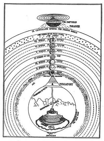

 ,
, , then the FLRW metric describes an infinite, “flat” Euclidean universe. If
  , then the metric describes an infinite, hyperbolic universe. If
  , though, the metric describes a finite universe: a 3-sphere.

