ANOTHER source of the sublime is infinity; if it does not rather belong to the last. Infinity has a tendency to fill the mind with that sort of delightful horror, which is the most genuine effect and truest test of the sublime.
Edmund Burke, A Philosophical Enquiry into the Origin of Our Ideas of the Sublime and Beautiful
Ask people for adjectives they would use to describe the infinite, and right after “really big” would probably come words like “overwhelming”, “incomprehensible”, “strange”. If they’re of a philosophical bent, the word “sublime” might even pass their lips.
In current common usage, “sublime” is most often used to mean something like “extremely good or beautiful”, but in philosophical aesthetics it has a different, more specific meaning. The modern philosophical study of the sublime began in the late 17th century but came to prominence in the 18th, most notably in the work of Edmund Burke and Immanuel Kant. For Burke and Kant, not only are sublimity and beauty distinct notions, but they are in fact mutually exclusive. In Kant’s analysis, a judgment of beauty is a pleasurable and disinterested cognition of a determinate form of a bounded object. If one finds a particular flower to be beautiful, then this is a judgment on the form of the flower: the coloration of its petals, the curl of its leaves, the way all of its components fit together into a harmonious whole. The sublime, on the other hand, is necessarily formless; it can only be conceived of as an overwhelming totality, and for Kant it is therefore a concept of reason rather than of cognition or understanding.
Kant distinguishes between two types of sublimity, each of which overwhelms us in a different way. The dynamical sublime occurs when one is confronted (from a sufficiently safe distance) with an overwhelming physical force, such as a powerful storm or a maelstrom at sea, bringing one’s physical finitude into stark relief. The mathematical sublime, which more directly concerns us here, occurs when one is confronted with something overwhelmingly large, something that outstrips one’s aesthetic comprehension of size. A large mountain, for instance, or a sprawling valley, or the vast reaches of outer space. And while there is a limit to our aesthetic comprehension of size, there are no such limits to our mathematical apprehension of size. For Kant, this movement from the initial inability to comprehend the totality to the subsequent recognition that it can nonetheless be apprehended is the essence of our experience of the sublime and the source of its pleasure.
(It is unsurprising that the notion of the sublime is often linked with that of the infinite, and it should be noted here that Kant was writing before the development of set theory and its accompanying array of sophisticated tools for making precise mathematical sense of the infinite in the 19th and 20th centuries. It is interesting to consider how a formal theory of the mathematical sublime might be affected by modern mathematical concepts, like the dizzying size of large cardinals, or the incompleteness and undecidability theorems of the mid-20th century.)
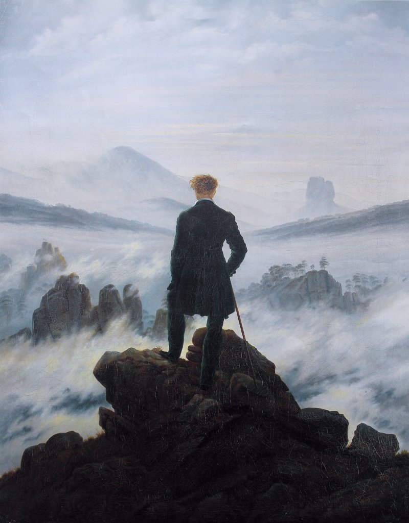
After Kant, the notion of the sublime continued to evolve, and it became a central topic of the work of 19th century Romantic artists. In the work of these artists, sublimity was no longer necessarily directly opposed to beauty, but it still drew much of its power from the juxtaposition of the overwhelming size or force of nature with the marked finitude, both physical and intellectual, of the human observer. Perhaps the artist of this era who is most associated with the sublime is the painter Caspar David Friedrich. Indeed, if I asked people to name a painting evoking the sublime, it is likely that the most common response would be his famous Wanderer above the Sea of Fog, depicting a man, his back to us, standing on a mountain precipice and looking out over a vast fog-covered landscape. Indeed, the scale of the vista, and the dense banks of fog obscuring the mysteries of the land below from human view, are quite evocative of the sublime. Yet the effect is somewhat mitigated by the positioning of the human observer in the painting, taking up a large space in the exact center of the canvas, artificially posed as if he is aware that his portrait is being painted. The depiction is not so much of somebody being swallowed up by the overwhelming grandeur of nature as of somebody confidently surveying his domain.
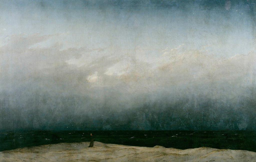
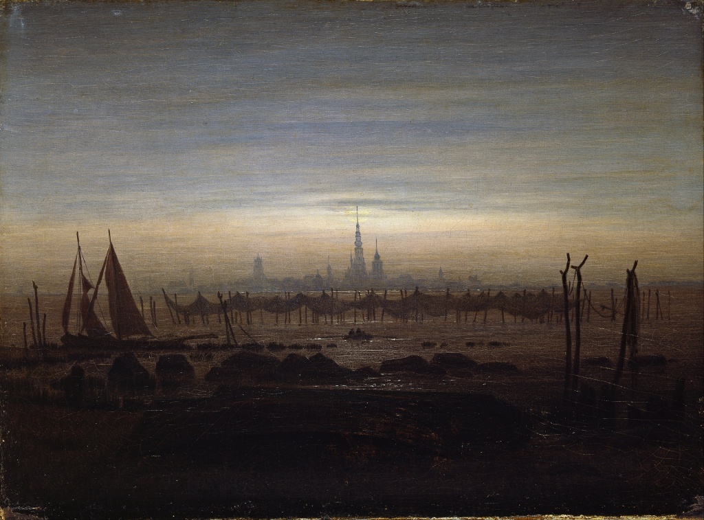
A different, slightly lesser known work by Friedrich is often held up as a more faithful representation of the sublime: The Monk by the Sea (see image below). Like Wanderer above the Sea of Fog, this painting depicts a solitary human in the midst of a vast landscape largely obscured by clouds or fog. Here, though, a formless sky takes up the majority of the painting, and the human figure (a monk on a beach, in this case) is much smaller and situated at the bottom of the painting, slightly left of center. His features and pose are quite indistinct; indeed, an inattentive viewer might not even see him, as his body blends into the sea behind him, and his head could be mistaken for one of its white-capped waves.
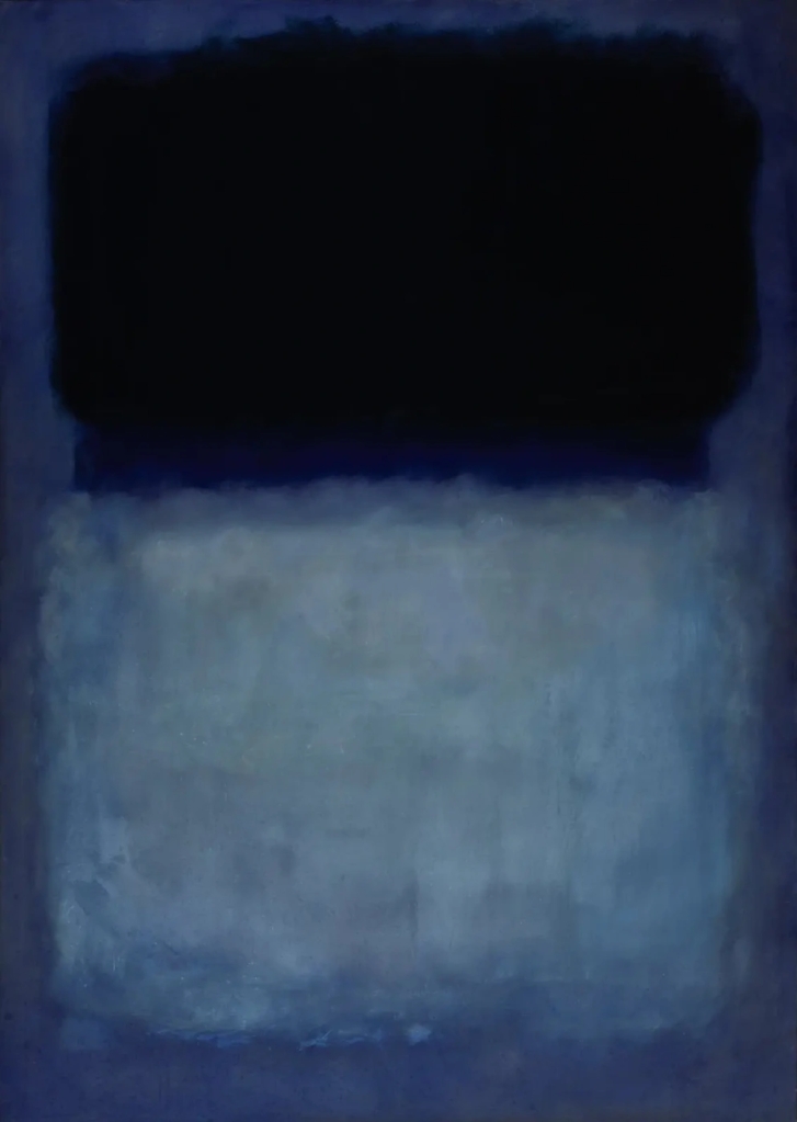
(A quick side note here. While the sublime is perhaps most tightly associated with 19th century Romantic art, it has been a central focus of a number of other artistic movements since then. Particularly prominent among these is the Abstract Expressionism of the 1940s-60s, with its massive canvases of abstract, almost formless color fields. Art historian Robert Rosenblum argued that the origins of Abstract Expressionism can be traced directly to Friedrich’s landscape painting, remarking quite perceptively, if a bit exaggeratedly, that one only has to remove the monk from Friedrich’s The Monk by the Sea to obtain Mark Rothko’s 1956 painting Untitled (Green on blue) (see image below). For a fuller exploration of the sublime in modern art, Rosenblum’s 1961 ARTnews article “The Abstract Sublime” is highly recommended (and contains the fantastic line, ‘What used to be pantheism has now become a kind of “paint-theism.”’).)
A couple of months ago, I gave a series of lectures at the Winter School in Abstract Analysis in Hejnice, Czech Republic. One of my title slides contained an image of Friedrich’s painting The Sea of Ice, which is the cover image for this post. I chose this painting both because of its affinities with the wintry landscape just outside our conference room and because the shape of the ice sheets jutting out from the sea in the painting is reminiscent of one of the mathematical arguments in the section of the lecture it preceded. The painting can also be seen as an effective depiction of the sublime, as the shipwreck in the right of the painting, almost swallowed up by the ice sheets, underscores the potential helplessness and insignificance of humankind in the face of the overwhelming power of nature, in this case encapsulated in the slow but irresistible movement of the massive ice sheets.
After the talk, I was approached by a mathematician who asked me if I knew the artist of the painting on my slides. I responded that yes, this was Caspar David Friedrich. He then asked if I knew what he and Caspar David Friedrich had in common. I replied that I did not, and he said that they shared a common birthplace, the small city of Greifswald, in northeast Germany on the Baltic Sea. He then told me that there was another relevant one-time resident of Greifswald: the mathematician Felix Hausdorff.
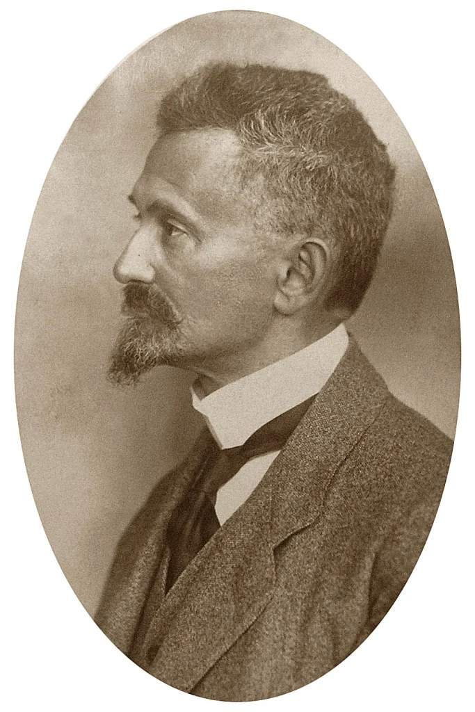
The name of Hausdorff is well-known to any student of topology, as his name adorns a number of fundamental concepts therein. He is considered one of the founders of topology and was also one of the key figures in the early development of set theory (out of which topology grew). In set theory, he is particularly remembered for his investigations of infinite ordered sets. He was the first to construct an example of a certain non-trivial ordered structure now known as a Hausdorff gap; such objects are still the topic of active research today. He is also remembered for his 1914 book Grundzüge der Mengenlehre (trans. Foundations of Set Theory), a copy of which adorns my office bookshelf. This was the first comprehensive book-length treatment of the still-young field of set theory and was very influential in its further development. It was mostly written in Greifswald, where Hausdorff served his first appointment at the rank of Full Professor from 1913 to 1921, in between appointments at the more bustling and mathematically well-connected University of Bonn. The mathematician I was speaking with suggested that Hausdorff needed to ditch the distractions of Bonn for the more tranquil surroundings of Greifswald in order to finish the Grundzüge der Mengenlehre (indeed, during the winter term of 1916/17, Hausdorff was the only mathematician at the University of Greifswald). And though the actual explanation probably has more to do with the mundane practical necessity for academics to take jobs where they can find them, it is also tempting to imagine Hausdorff purposefully seeking out the birthplace of Caspar David Friedrich as a setting in which to contemplate infinity and compose his magnum opus.
Cover image: The Sea of Ice (1823-24) by Caspar David Friedrich
While trying to understand Kant’s conception of the sublime and its connection with art, I found the following two articles helpful:
“The Copernican Turn in Aesthetics: How Kant’s Notion of the Mathematical Sublime Re-Aestheticizes the Universe” by Thiti Owlarn
“The Simplicity of the Sublime: A New Picturing of Nature in Caspar David Friedrich” by Laure Cahen-Maurel
 , is of course a finite set. The set
  is finite, as it contains 4 elements (the single-digit prime numbers). And the set
  is finite, containing only 2 elements (the set of natural numbers and the set of real numbers). And while all three of these are certainly finite sets, two of them seem more truly finite than the other. The empty set is obviously finite through and through, as is the set
  , since it only has finitely many elements and each of those elements is simply a finite number. It feels a bit like cheating, on the other hand, to call
  is truly finite if it satisfies the following two properties:
 ? This set is finite, having two elements (
 and
and  ). And each of its elements is finite, having only one element (
 and
and  , respectively). So
  satisfies this definition but again should not be considered to be truly finite. We want to somehow catch our tail and say that a set is truly finite if, no matter how many layers deep you go into the set, you never reach an infinite set. Something like:
 . It has one element, so it is finite. Moreover, we now know that its one element, the empty set, is hereditarily finite. Therefore,
  ? It has two elements, so it is finite. Moreover, we have already seen that both of its elements,
  or
or  or
or  . Our apparently circular definition actually has an abundance of unambiguous examples.
 denote the set of all elements of elements of
  denote the set of all elements of elements of
  is infinite, then stop the process and conclude that
  denote the set of all elements of elements of
  , one of our examples of a hereditarily finite set from above, and run the above process. In Step 0, we note that
  , and continue to Step 2.
 , and continue to Step 3.
 be the set of all elements of elements of
  , and continue to Step 4.
 , a set that we definitely didn’t want to consider hereditarily finite. In Step 0, we note that
  , and continue to Step 2.
 , and continue to Step 3.
 of
of  .
. , i.e., the set whose only element is itself. Let’s see what happens if we try to apply our process to
  . But
. But  . We continue to Step 2.
 is finite, as it contains only three elements. This intuitive understanding of “finite” and “infinite” works fine in everyday practice, but it does not amount to a definition, and if we want to study sets generally rather than specific instances of sets, or if we want to study the notion of “infinity”, then it will be important to have a solid definition of the concept “finite set”. And, considering that this is a concept that we are all quite familiar with, this turns out to be surprisingly tricky.
 and
and  have the same size if their elements can be put into a one-to-one correspondence with one another. Now, when you think about a finite set, you probably think about the act of counting the elements in the set, and eventually completing this count. What do you use to count the elements of the set? The natural numbers! (Recall that natural numbers are whole numbers of the form
  .) A finite set should thus be a set whose size is the same as some natural number. This might lead us to formulate the following attempted definition:
 , find a set
  that is not an element of
  is the size of the set
  formed by adding
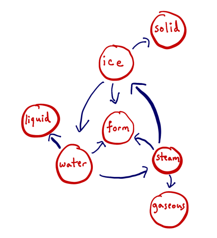
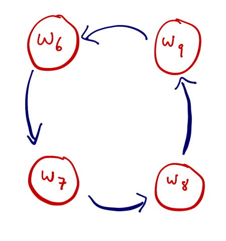
 and so on. Recalling the meaning of the graph, this means that the definition of
  contains
  , the definition of
  , and so on.
 visited in our path itself has a definition, and therefore there are certainly arrows pointing out of the node associated with
  .
. such that
  and
and  is the same word as
  . But in that case, look at what we have:
 ;
; ;
; ;
; ).
).
 and
and 
 , a subgraph
  of
of 
 , is the least number of colors needed for a chromatic coloring of
  . It is not hard to show (Exercise: check this!) that it is impossible to construct a chromatic coloring of
  . Notice that the chromatic number of a graph
  is a finite number, and, for every finite subgraph
  . Then
  .
. from the natural numbers to the natural numbers by letting
  be the least number of vertices in a subgraph of
  .
. for every natural number
  , then
  . This is because, if
  is a finite subgraph of
  , then, by removing vertices from
  with chromatic number
  .
. , that means that any subgraph of
  is larger than the number of atoms in the observable universe, and
  is inconceivably larger still. Intuitively, the faster
  such if
  . All larger cardinalities are said to be uncountable. The smallest uncountable cardinal is
  , the next smallest is
  , and so on.
 and
and  for all
  ).
). and
and  , which is a strengthening of the Continuum Hypothesis. They then perform a technique known as forcing to produce a model of set theory in which the E-H-S question has a positive answer. While their ideas ended up not being useful for the technical problem I was working on, while reading their proof, I had a vague feeling that I could combine some of their ideas with some ideas I had developed the previous fall to show that the forcing step of their proof was unnecessary. In other words, it seemed that maybe a positive answer to the E-H-S question already followed from
 . This is a truly astounding number, dwarfing the estimated number of atoms in the observable universe (
 ) or the estimated number of legal positions in chess (a piddling
  ). The possibilities in go are, for all intents and purposes, infinite. No matter how much one learns, one knows essentially nothing.
 that cannot be reached from below through the standard procedures of climbing to the next cardinal, applying cardinal exponentiation, or taking unions of a small number of small sets. (More formally,
  , we have
  .)
.)
 ,
,
 ,
,
 ,
,

 approach a fixed number
  as
as  .
.
 . The lamp is half on and half off.
 .
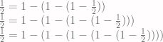
. in for
  on the right side of this equation, he finds that
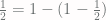 .
. .
. .
. ,
, as above. Instead, one computes the limit of the average of the first
  and initial sums
  , one then defines a sequence
  by letting
 .
. approach a fixed number
  .
.