Introducing The Humming of the Strings

Hello! I’m sorry that I haven’t been around much in the last few months, which have been rather busy for me. I’m hoping to continue more regular posting now, though, starting with the announcement of a new project: Point at Infinity‘s first spin-off blog, The Humming of the Strings.

Loyal readers will remember a few posts here on Point at Infinity about music. We had a post about the Shepard tone, an aural illusion that seems to perpetually rise in pitch, two posts about the Risset rhythm, the Shepard tone’s rhythmic cousin, and a post about Euclidean rhythms and their surprising connections with nuclear physics, computer graphics, and the Hebrew calendar. These were among the most enjoyable posts for me to write, and some of them were among the favorites of readers as well. Mathematics and music are two passions of mine, and there is a vast field of ideas to explore here, many of which don’t necessarily fit here on Point at Infinity. This is why I’m starting The Humming of the Strings, to provide a place for more in-depth exploration of musical topics that might be out of place here.

There is another, more technical reason for this blog. Over the last couple of years, I’ve sporadically been playing around with SuperCollider, an audio synthesis platform and programming language. It is a wonderful tool for exploring the connections between math and music, and I plan on using it to create music and audio samples for The Humming of the Strings, and on sharing what I learn in this process with the readers. I’m hoping that the details of the computer programming will be of interest to some readers, and I will try to make it as unintrusive as possible for those readers not interested in it. (I’m anticipating that most posts will consist of a non-technical body section followed by a technical appendix with details of the code.)

I hope you will join me over at The Humming of the Strings. I will likely primarily be posting there rather than here in the near future, though there may be some new content on Point at Infinity from time to time. Thanks for reading, and Happy New Year!

L’escalier du Diable

Welcome one, welcome all to the Point at Infinity sideshow, where today we present a tantalizing and diabolical selection of musical and mathematical curiosities. Just watch your step; these stairs can be a bit tricky.

---

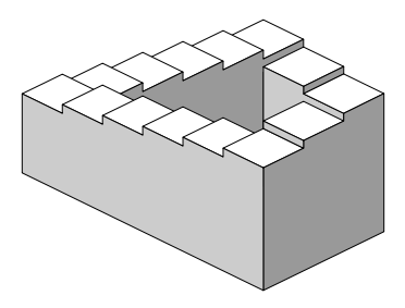
A few months ago, you may recall, we published two posts about the Shepard tone and the Risset rhythm, aural illusions in which a tone or rhythm seems to perpetually rise or fall in pitch or in tempo but is actually repeating the same pattern over and over again, the musical equivalents of Penrose stairs.

Penrose stairs. (Image in the public domain.)

To accompany the posts we created some sound samples so the readers could hear the illusions themselves. A couple of weeks ago, one of these samples was used in an internet radio program on audio paradoxes released by Eat This Radio, paired with some work of Jean-Claude Risset. The entire program is really excellent, ranging from a piece by J.S. Bach to mid-twentieth century audio experiments to modern electronic music, and I encourage all of you to listen to it.

---

One of the pieces in the radio program is a piano étude written by György Ligeti in the late twentieth century. The étude is named L’escalier du diable, or The Devil’s Staircase, and its repeated ascents of the keyboard have a striking resonance with the never-ending ascent of the Shepard tone.

---

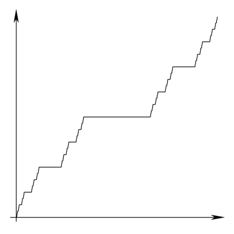
The Devil’s Staircase is also the colloquial name given to a particular mathematical function introduced by Georg Cantor in the 1880s. It is a function defined on the set of real numbers between 0 and 1 and taking values in the same interval, and it has some quite curious properties. Before we discuss it, let’s take a look at (an approximation to) the graph of the function.

Graph of the Devil’s Staircase. By Theon, CC BY-SA 3.0.

To appreciate the strangeness of this function, let us recall some definitions regarding functions of real numbers. Very roughly speaking, a function is called continuous if it has no sudden jumps, or if its graph can be drawn without lifting the pencil from the page. Continuous functions satisfy a number of nice properties, such as the intermediate value theorem.

The derivative of a function at a given point of its domain, if it exists, measures the rate of change of the function at that point. If the x-axis measures time and the y-axis measures the position of an object along some one-dimensional track, then the derivative can be thought of as the velocity of that object. If a function is differentiable at a point (i.e., if its derivative exists there) then it must be continuous at that point, but the converse is not necessarily true. (For example, if the graph of a function has a sharp corner at a point, then the function cannot be differentiable there.)

Let’s think about what it means for a function to have a derivative of 0 at a point. It means that, at that point, the rate of change of the function has vanished. It means that, if we zoom in sufficiently close to that point, the function should look like a constant function. Its graph should look like a horizontal line. What would it mean for a function to have a derivative of 0 almost everywhere? (Here “almost everywhere” is a technical term (which I’m not going to define) and not just me being vague.) One might think that this must imply that the function is a constant function. At almost every point in its domain, the rate of change of the function is 0, so how can the value of the function change?

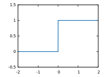
One will quickly discover that this is not quite right. Consider the function defined on the real numbers whose value is 0 at all negative numbers and 1 at all non-negative numbers.

This function has derivative 0 everywhere except at 0 itself, and yet it increases from 0 to 1. It does this quite easily by being discontinuous at 0, which, in hindsight, seems sort of like cheating. So what if we also require our function to be continuous? Now we need more exotic examples, and this is where the Devil’s Staircase comes in, for the Devil’s Staircase is a continuous function, it is differentiable almost everywhere, it has a  derivative of 0 wherever its derivative is defined, and yet it still manages to increase from 0 to 1. Wild!

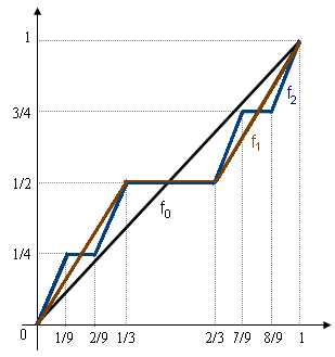
What is the Devil’s Staircase exactly? I’ll give two different definitions. The first proceeds via an iterative construction. Start with the function . Its graph, between 0 and 1, is simply a straight line segment increasing from (0,0) to (1,1). Now, look at the midpoint of this increasing line segment, and draw a horizontal line segment centered there whose length is 1/3 of the horizontal line of the original increasing segment. Now connect the ends of this line segment via straight lines to (0,0) and (1,1). This new curve is the graph of a function that we call . It consists of two increasing line segments with one horizontal line segment between them. Now repeat the process that took us from to on each of these increasing line segments, and let be the function whose graph is the result. Continue in this manner, constructing for every natural number .

First three steps of the iterative construction of the Devil’s Staircase. (Image in the public domain.)

It turns out that, as goes to infinity, the sequence of functions converges (uniformly) to a single function. This function is the Devil’s Staircase.

A more direct but also more opaque definition is as follows: Given a real number between 0 and 1, first express in base 3 (i.e., using only 0s, 1s, and 2s). If this base 3 representation contains a 1, then replace every digit after the first 1 with a 0. Next, replace all 2s with 1s. The result has only 0s and 1s, so we can interpret it as a binary (i.e., base 2) number, and we let be this value. Then the function defined in this manner is the Devil’s Staircase. Play around with this definition, and you might get a feel for what it’s doing.

---

And now, on our way out, some musical addenda. An encore, if you will. First, after making the Risset rhythms for the aforementioned post, I did some further coding and wrote a little program that can take any short audio snippet and make a Risset rhythm out of it. Here’s an example, first accelerating and then decelerating, using a bit from a Schubert piano trio.

You may recognize the sample from the soundtrack to Barry Lyndon.

Finally, I can’t help but include here one of my favorite pieces by Ligeti, Poema sinfónico para 100 Metrónomos.

---

Cover image: Devil’s Staircase Wilderness, Oregon, USA

Beats by Bjorklund

You gotta keep ’em separated.

-The Offspring, “Come Out And Play”

(Friendly note to the reader before we begin: If you’re looking for music to listen to while reading this post, just scroll to the bottom…)

The Spallation Neutron Source (SNS), at Oak Ridge National Laboratory in Tennessee, provides the world’s most intense pulsed neutron beams for scientific research. By accelerating proton pulses and directing them towards a mercury target, the laboratory ejects neutrons from the target. By measuring the energies and angles of these scattered neutrons, scientists can uncover information about the magnetic and molecular structure of various materials.

Pulses at the SNS are grouped into super-cycles, each 10 seconds long and consisting of 600 pulses. Commonly, experimenters will want to perform a particular action on a fixed number of pulses (, say) during each super-cycle and will want to have the executions of the actions spaced as evenly as possible across time. If evenly divides 600, then the solution to this problem is trivial: just perform the action on pulses . If does not evenly divide 600, though, then the solution is not as obvious.

This is of course a special case of a general problem: Given cycles of length , how can events be spaced as evenly as possible across a single cycle? (Naturally, we should have here.) As seen above, the problem is trivial if evenly divides , so we shall assume this is not the case. In fact, we shall assume that and are relatively prime, i.e., that they have no common positive divisors other than 1. We will also assume that , since it is also trivial to evenly distribute one event across a cycle.

This exact problem was tackled by E. Bjorklund, motivated by timing questions at the SNS. In this paper, he presents an algorithm for generating solutions. For ease of notation, let us denote a cycle by a sequence of 0s and 1s, with a 1 representing an event taking place and a 0 representing an event not taking place. For definiteness, we will always start the sequence with a 1, but, because we are dealing with cyclic phenomena, we will consider two “rotations” of the same base sequence to be the same. For example, we consider 10010 and 10100 to be the same, since the second is just the first “rotated” (and wrapped around) three spaces to the right.

We will not give a formal account of Bjorklund’s algorithm here, but we will illustrate it with an example that we hope will indicate how to carry it out in general. Suppose we are given the specific problem of evenly spacing eight events in a cycle of length thirteen. Our final sequence will thus have eight 1s and five 0s. We start with thirteen individual sequences, each of length one, with all of the 1s first and then all of the 0s:

[1] [1] [1] [1] [1] [1] [1] [1] [0] [0] [0] [0] [0]

You will notice that we have two different sequences in this list ([1] and [0], here). This will be true for every step of the algorithm. In the next step, we take all instances of the second sequence ([0], here) and append them in turn to instances of the first sequence. Since there are five instances of the second sequence, five instances of the first sequence will become longer, and we obtain:

[10] [10] [10] [10] [10] [1] [1] [1]

We again have two different sequences ([10] and [1]). And we again take all instances of the second sequence and append them in turn to instances of the first sequence, obtaining:

[101] [101] [101] [10] [10]

Repeating this process again yields:

[10110][10110][101]

Technically, since there is only one instance of the second sequence in this stage, we could stop here and just append all of the sequences in order to obtain the correct solution, but let us continue for illustration’s sake. Next, we get:

[10110101][10110]

And, finally:

[1011010110110}

(which is just a rotation of what we would have gotten two stages earlier: [1011010110101]). Thus, the optimal way of evenly distributing eight events in a single cycle of length 13 is given by the sequence 1011010110110. A similar process will yield the correct answer in any other specific instance of this problem.

(The astute reader might have noticed that this algorithm bears a resemblance to Euclid’s famous algorithm for calculating the greatest common divisor of two positive integers. This is not a coincidence.)

---

You might be slightly disturbed by my lack of rigor at this point. Indeed, there are two ways in which I am slightly cheating the reader. First, I have not really said what I mean by having events be spaced “as evenly as possible.” Intuitively, 1011010110110 is more even than 111111110000, or 1101101101100, or, if one thinks about it, 1011011011010, but how do we know it is “as even as possible,” and what do we even mean by this? Second, even if I had given a rigorous definition of “evenness,” I have not proven that Bjorklund’s algorithm does in fact deliver the optimal result (again, this should be intuitively plausible, but should perhaps not be blindly accepted). I will do neither of these things here, but will instead direct the interested reader to the excellent paper, “The distance geometry of music,” by Demaine, Gomez-Martin, Meijer, Rappaport, Taslakian, Toussaint, Winograd, and Wood, from which much of this post was derived.

---

Unsurprisingly, the problem of evenly distributing events or items into cycles of length does not show up only in nuclear physics. Let us briefly look at a couple of other interesting appearances.

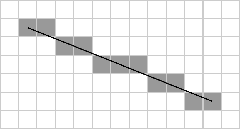
Computer graphics: Suppose you want to depict a straight line on a computer screen with a slope of . Computer screens consist of grids of pixels, so, unless the line is horizontal or vertical, it cannot be drawn perfectly straight. Here is an example of a segment of a line with slope :

A line with slope -5/11, superimposed over a pixel approximation. Created by Crotalus horridus, Public Domain

It should be clear that, at least as long as , the problem of drawing this line consists of choosing out of every horizontal spaces after which to move your line one space vertically. To make your line as straight as possible, this distribution should be as even as possible. Indeed, the situation depicted above can be represented by the sequence 10101001010, where 1 indicates a vertical shift and 0 represents the absence of a vertical shift. This is precisely the result one gets (after a rotation) if one applies Bjorklund’s algorithm to the numbers 5 and 11.

Leap year distribution: The problem of reconciling the fact that one revolution of the earth around the sun does not take an exact integer number of days with the desire to have years that last an exact integer number of days is one that affects every calendar design. It is handled particularly interestingly in the Hebrew calendar. The Hebrew calendar is a lunisolar calendar, in which each month lasts one full cycle of the moon, but in which adjustments are made so that each month occurs at roughly the same stage of the solar year during each cycle. The Hebrew calendar reconciles these two contradictory demands by having twelve months in a typical year but, during certain “leap years,” having one of these months (namely, Adar) repeated to yield a year of thirteen months. It turns out that, to keep the Hebrew calendar very close to being in sync with the solar cycles, one needs to have seven out of every nineteen years be leap years. It is also natural to want these leap years to be spaced as evenly as possible. And, indeed, the distribution of these seven leap years in nineteen-year cycles in the Hebrew calendar is given precisely by a rotation of the result of Bjorklund’s algorithm applied to the numbers seven and nineteen.

---

Perhaps the most interesting appearances of the problem of evenly distributing events in a cycle, though, are in music. If one thinks of a musical measure consisting of beats as being a cycle of length , of a 1 as being a note being played, and of a 0 as being the absence of a note being played, then our strings of 1s and 0s can be thought of as musical rhythms. And it turns out that applications of Bjorklund’s algorithm, when interpreted in this way, yield a startling variety of musical rhythms used in practice around the world. We end this post by presenting a few prominent examples.

In what follows, we notationally replace 1s with ‘x’s and 0s with dots. This is more conducive to following along with musical rhythms, as it is visually easier to get lost in strings of 1s and 0s than in strings of ‘x’s and dots. An ‘x’ thus denotes a note being played and a dot denotes the absence of a note being played (or, often, an ‘x’ denotes an accented beat and a dot denotes an unaccented beat).  Given numbers , we denote by the result of Bjorklund’s algorithm applied to and . The sequence that follows is the rotation of this result that is actually heard in the piece of music. As before, we restrict ourselves to the interesting cases in which and are relatively prime and . (Of course, the standard waltz rhythm [x .  . ], for example, would be E(1,3), and the standard backbeat rhythm [. x . x ] would be a rotation of E(2,4), but these are sort of boring in this context.)

There’s some good music here. Enjoy!

E(2,5) – (x . . x . ): “Take Five” by The Dave Brubeck Quartet.

E(3,7) – (x . x . x . . ): “Money” by Pink Floyd.

E(3,8) – (x . . x . . x . ): This is the famous tresillo rhythm, which can be heard throughout Latin American and sub-Saharan African music as well as in such songs as “Hound Dog,” “Despacito,” and the song we feature here, “Intro” by The xx.

E(5,8) – (x . x x . x x . ): This is the cinquillo rhythm, an elaboration of the tresillo that is also ubiquitous in Latin American and sub-Saharan African music. It also features prominently in “Come Out and Play” by The Offspring.

E(4,9) – (x . x . x . x . . ): This is our second track from the classic Time Out album, which was inspired by musical styles (especially time signatures) observed during travels in Europe and Asia. Brubeck saw this particular beat being played by Turkish street musicians and then used it for  “Blue Rondo à la Turk” by The Dave Brubeck Quartet.

E(4,11) – (x . . x . . x . . x . ): “Outside Now” by Frank Zappa.

E(5,11) – (x . x . x . x . x . .): “Promenade” from Pictures at an Exhibition by Modest Mussorgsky.

E(7,12) – (x . x . x x . x . x . x): This is one of the most important rhythms in sub-Saharan Africa, often used as a bell pattern. It is also a common beat in the Palo music of the Caribbean. It can be heard played by the claves player in this performance by Los Calderones, which I have been listening to non-stop for the last hour. (Note also that, if one re-interprets this sequence in a harmonic rather than rhythmic setting, in which each step of the cycle represents a half-step in pitch, an ‘x’ represents the inclusion of that note in a scale, and a dot represents the exclusion of that note from a scale, then this sequence (this exact rotation, in fact) precisely corresponds to the major diatonic scale, the most common musical scale in Western music!)

E(4,13) – (x . . x . . x . . x . . . ): This rhythm can be heard in the instrumental sections of “Golden Brown” by The Stranglers.

E(5,16) – (x . . x . . x . . . x . . x . . ): This rhythm forms the basis for much bossa nova music and, when significantly slowed down, “Pyramid Song” by Radiohead.

---

Cover image: Detail from “Wall Drawing #260” by Sol LeWitt